工具使用-PlotNeuralNet 绘制漂亮深度网络图

github 链接 https://github.com/HarisIqbal88/PlotNeuralNet

项目提供了python的接口，但python接口感觉不是很好用，所以我最终选择直接使用latex接口。

下载项目

1	git clone https://github.com/HarisIqbal88/PlotNeuralNet

如果使用Latex绘图的话，只需要layers文件夹就足够了。

自定义绘图单元

项目定义了3种绘图单元：Ball.sty, Box.sty和RightBandedBox.sty. 其中Ball.sty 主要用来表示concat操作，比如element-wise add或者multiple，或者correlation等操作。 Box.sty 是一个3D box形状，一般可以用来表示conv， pool，等单独的tensor操作。 RightBandedBox同样是3Dbox 形状，和Box.sty的不同点在于它分为主体部分和右边的banded部分，想象其表示conv+relu整体的模块。

我们直接分析examples/fcn8s/fcn8.tex中的代码，看看如何通过.tex文件绘制网络结构。

\documentclass[border=15pt, multi, tikz]{standalone}
\usepackage{import}
\subimport{../../layers/}{init}  % 通过init导入自己定义的绘图单元
\usetikzlibrary{positioning}
\usetikzlibrary{3d} %for including external image 

% 下面6行定义了将要使用的6种结构的表示颜色， 如Conv， ReLU， Pool， Deconv等
\def\ConvColor{rgb:yellow,5;red,2.5;white,5}
\def\ConvReluColor{rgb:yellow,5;red,5;white,5}
\def\PoolColor{rgb:red,1;black,0.3}
\def\DcnvColor{rgb:blue,5;green,2.5;white,5}
\def\SoftmaxColor{rgb:magenta,5;black,7}
\def\SumColor{rgb:blue,5;green,15}

\begin{document}
\begin{tikzpicture}
\tikzstyle{connection}=[ultra thick,every node/.style={sloped,allow upside down},draw=\edgecolor,opacity=0.7]
%%%%%%%%%%%%%%%%%%%%%%%%%%%%%%%%%%%%%%%%%%%%%%%%%%%%%%%%%%%%%%%%%%%%%%%%%%%%%%%%%%%%%%%%
%% Draw Layer Blocks， 开始绘制网络， 首先是绘制网络中每一个结构，然后再将结构连接
%%%%%%%%%%%%%%%%%%%%%%%%%%%%%%%%%%%%%%%%%%%%%%%%%%%%%%%%%%%%%%%%%%%%%%%%%%%%%%%%%%%%%%%%
% 定义一个node， 在（-3， 0， 0）位置绘制图像， 2D图像对应映射到zy平面。
% 注意这里的坐标系采用的是左手坐标系，具体而言右向是x正轴， 向上是y正轴，往远方是z正轴
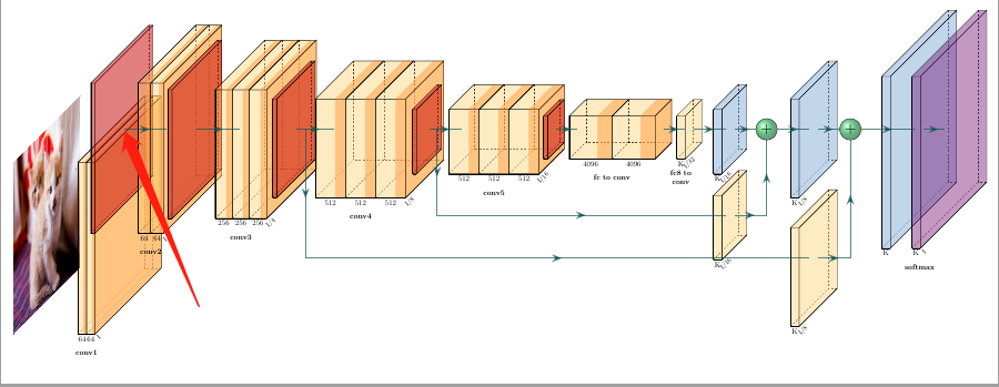
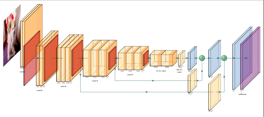
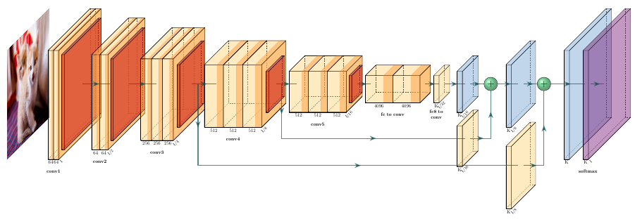
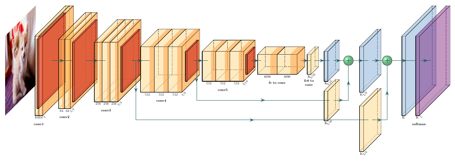
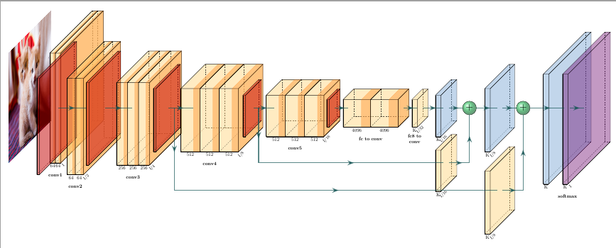
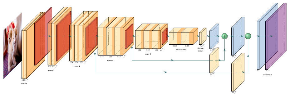
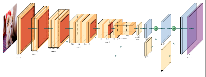
\node[canvas is zy plane at x=0] (temp) at (-3,0,0) {\includegraphics[width=8cm,height=8cm]{cats.jpg}};
% conv1_1,conv1_2,%pool1
% 绘制卷积层， at (0,0,0)表示从空间坐标原点开始， shift表示相对于 at的点的位移， 最终开始绘制的结构中心点坐标是 at+shift, RightBandedBox 表示这是conv+relu结构， RightBandedBoxd的name=cr1， 其标题是con1， 标题一般写在结构的下方，见示意图。xlabel， ylabel， zlabel分别是在3Dbox三个方向边上的label， 这里xlabel中有两个str 是由于width内有两个数值，表示x方向分成两部分， width则分别表示两部分的width， fill表示3D box的填充颜色， bandfill表示banded部分的填充颜色， depth是指z轴方向的长度。
\pic[shift={(0,0,0)}] at (0,0,0) {RightBandedBox={name=cr1,caption=conv1,%
        xlabel={{"64","64"}},zlabel=I,fill=\ConvColor,bandfill=\ConvReluColor,%
        height=40,width={2,2},depth=40}};
% 这里新出现的是 cr1-east 表示的是， cr1结构的最右面， 上北下南，左西右东， 除了东南西北还有near表示z轴最小的那面，也就是离我们最近的那面，同理far表示离我们最远的那一面， anchor则表示在cr1的中心点位置， 另外任意两个可能的组合都行，比如northwest， 但有些组合不行比如northsouth。 效果图见图1, 新出现的属性opacity=0.5， 默认的上文定义opacity=0.75，所以pool层的透明度更低。
\pic[shift={(0,0,0)}] at (cr1-east) {Box={name=p1,%
        fill=\PoolColor,opacity=0.5,height=35,width=1,depth=35}};
% conv2_1,conv2_2,pool2
% conv2的结构在p1-east基础上右移两个单位 shift={(2, 0, 0)}
\pic[shift={(2,0,0)}] at (p1-east) {RightBandedBox={name=cr2,caption=conv2,%
        xlabel={{"64","64"}},zlabel=I/2,fill=\ConvColor,bandfill=\ConvReluColor,%
        height=35,width={3,3},depth=35}};
\pic[shift={(0,0,0)}] at (cr2-east) {Box={name=p2,%
        fill=\PoolColor,opacity=0.5,height=30,width=1,depth=30}};
% conv3_1,conv3_2,pool3
\pic[shift={(2,0,0)}] at (p2-east) {RightBandedBox={name=cr3,caption=conv3,%
        xlabel={{"256","256","256"}},zlabel=I/4,fill=\ConvColor,bandfill=\ConvReluColor,%
        height=30,width={4,4,4},depth=30}};
\pic[shift={(0,0,0)}] at (cr3-east) {Box={name=p3,%
        fill=\PoolColor,opacity=0.5,height=23,width=1,depth=23}};
% conv4_1,conv4_2,conv4_3,pool4
\pic[shift={(1.8,0,0)}] at (p3-east) {RightBandedBox={name=cr4,caption=conv4,%
        xlabel={{"512","512","512"}},zlabel=I/8,fill=\ConvColor,bandfill=\ConvReluColor,%
        height=23,width={7,7,7},depth=23}};
\pic[shift={(0,0,0)}] at (cr4-east) {Box={name=p4,%
        fill=\PoolColor,opacity=0.5,height=15,width=1,depth=15}};
% conv5_1,conv5_2,conv5_3,pool5
\pic[shift={(1.5,0,0)}] at (p4-east) {RightBandedBox={name=cr5,caption=conv5,%
        xlabel={{"512","512","512"}},zlabel=I/16,fill=\ConvColor,bandfill=\ConvReluColor,%
        height=15,width={7,7,7},depth=15}};
\pic[shift={(0,0,0)}] at (cr5-east) {Box={name=p5,%
        fill=\PoolColor,opacity=0.5,height=10,width=1,depth=10}};    
%% fc6, fc7 -> cr6, cr7
\pic[shift={(1,0,0)}] at (p5-east) {RightBandedBox={name=cr6_7,caption=fc to conv,%
        xlabel={{"4096","4096"}},fill=\ConvColor,bandfill=\ConvReluColor,%
        height=10,width={10,10},depth=10}};  
%% fc8 -> cr8 (score32)
% 单独并以conv层的时候，也是绘制的box块，和pool层不同的是颜色
\pic[shift={(1,0,0)}] at (cr6_7-east) {Box={name=score32,caption=fc8 to conv,%
        xlabel={{"K","dummy"}},fill=\ConvColor,%
        height=10,width=2,depth=10,zlabel=I/32}};
%%%%%%%%%%%%%%%%%%%%%%%%%%%%%%%%%%%%%%%%%%%%%%%%%%%%%%%%%%%%%%%%%%%%%%%%%%%%%%%%%%%%%%%%
%%Joining with previous streams (fcn-16s)
%% Upsampling Deconv Layer
%% Dcnv32    
% 这里xlabel中的dummy加不加效果是一样的
\pic[shift={(1.5,0,0)}] at (score32-east) {Box={name=d32,%
        xlabel={{"K","dummy"}},fill=\DcnvColor,%
        height=15,width=2,depth=15,zlabel=I/16}};  
%% score16
% 注意这里的位置是d32-west是为了保证score16和d32是左对齐的
\pic[shift={(0,-4,0)}] at (d32-west) {Box={name=score16,%
            xlabel={{"K","dummy"}},fill=\ConvColor,%
            height=15,width=2,depth=15,zlabel=I/16}};
%% Elementwise sum between score16 and up32
% 引入了新的结构 Ball， radius定义了Ball的大小， logo是ball中的文字， 可以替换成$*$等
\pic[shift={(1.5,0,0)}] at (d32-east) {Ball={name=elt1,%
        fill=\SumColor,opacity=0.6,%
        radius=2.5,logo=$+$}};
%%%%%%%%%%%%%%%%%%%%%%%%%%%%%%%%%%%%%%%%%%%%%%%%%%%%%%%%%%%%%%%%%%%%%%%%%%%%%%%%%%%%%%%%
%%Joining with previous streams (fcn-8s)
%% Upsampling Deconv Layer
%% Dcnv16    
\pic[shift={(1.5,0,0)}] at (elt1-east) {Box={name=d16,%
        xlabel={{"K","dummy"}},fill=\DcnvColor,%
        height=23,width=2,depth=23,zlabel=I/8}};  
%% score8
\pic[shift={(0,-6,0)}] at (d16-west) {Box={name=score8,%
        xlabel={{"K","dummy"}},fill=\ConvColor,%
        height=23,width=2,depth=23,zlabel=I/8}};
%% Elementwise sum between score16 and up32
\pic[shift={(1.5,0,0)}] at (d16-east) {Ball={name=elt2,%
        fill=\SumColor,opacity=0.6,%
        radius=2.5,logo=$+$}};
%%%%%%%%%%%%%%%%%%%%%%%%%%%%%%%%%%%%%%%%%%%%%%%%%%%%%%%%%%%%%%%%%%%%%%%%%%%%%%%%%%%%%%%%%    
%%% Output
%%%%%%%%%%   
%% Dcnv8    
\pic[shift={(2.5,0,0)}] at (elt2-east) {Box={name=d8,%
        xlabel={{"K","dummy"}},fill=\DcnvColor,%
        height=40,width=2,depth=40}}; 
%%%%%%%%%%   
%% softmax    
\pic[shift={(1,0,0)}] at (d8-east) {Box={name=softmax,caption=softmax,%
        xlabel={{"K","dummy"}},fill=\SoftmaxColor,%
        height=40,width=2,depth=40,zlabel=I}}; 
%%%%%%%%%%%%%%%%%%%%%%%%%%%%%%%%%%%%%%%%%%%%%%%%%%%%%%%%%%%%%%%%%%%%%%%%%%%%%%%%%%%%%%%%
%% Draw connections
% 在每一个结构都绘制完成后，连接结构
%%%%%%%%%%%%%%%%%%%%%%%%%%%%%%%%%%%%%%%%%%%%%%%%%%%%%%%%%%%%%%%%%%%%%%%%%%%%%%%%%%%%%%%%
% 下面7行就是直接连接不同的结构
\draw [connection]  (p1-east)    -- node {\midarrow} (cr2-west);
\draw [connection]  (p2-east)    -- node {\midarrow} (cr3-west);
\draw [connection]  (p3-east)    -- node {\midarrow} (cr4-west);
\draw [connection]  (p4-east)    -- node {\midarrow} (cr5-west);
\draw [connection]  (p5-east)    -- node {\midarrow} (cr6_7-west);
\draw [connection]  (cr6_7-east)   -- node {\midarrow} (score32-west);
\draw [connection]  (score32-east) -- node {\midarrow} (d32-west);
% 值得注意的是下面绘制分支的过程。
% 下行表示在 p4-east 到 cr5-west的路线中， 选择0.25的部分创建一个新的点 称为 between4_5
\path (p4-east) -- (cr5-west) coordinate[pos=0.25] (between4_5) ;
% 从新创建的点绘制折线到score16-west，分为两段，第一段是由between往下， 然后再由转折点绘制到score16-west. 这里score16-west -| between4_5 表示between4_5在score16-west的中心点法线上的垂足， 不能交换位置， between4_5 -| score16-west则表示score16-west中心点在between4_5x方向射线上的垂足。
\draw [connection]  (between4_5)    -- node {\midarrow} (score16-west-|between4_5) -- node {\midarrow} (score16-west);
\draw [connection]  (d32-east) -- node {\midarrow} (elt1-west);
% 类似的，这里的score16-east -| etl1-south 表示etl1-south点在score16-east射线的垂足
\draw [connection]  (score16-east) -- node {\midarrow} (score16-east -| elt1-south) -- node {\midarrow} (elt1-south);
\draw [connection]  (elt1-east) -- node {\midarrow} (d16-west);

\path (p3-east) -- (cr4-west) coordinate[pos=0.25] (between3_4) ;
\draw [connection]  (between3_4) -- node {\midarrow} (score8-west-|between3_4) -- node {\midarrow} (score8-west);
\draw [connection]  (d16-east) -- node {\midarrow} (elt2-west);
\draw [connection]  (score8-east) -- node {\midarrow} (score8-east -| elt2-south)-- node {\midarrow} (elt2-south);
\draw [connection]  (elt2-east) -- node {\midarrow} (d8-west);
\draw [connection] (d8-east) -- node{\midarrow} (softmax-west);
%%%%%%%%%%%%%%%%%%%%%%%%%%%%%%%%%%%%%%%%%%%%%%%%%%%%%%%%%%%%%%%%%%%%%%%%%%%%%%%%%%%%%%%%

\end{tikzpicture}
\end{document}\grid

north

cr1-north

south

cr1-south

east

cr1-east

west

cr1-west

near

cr1-near

far

cr1-far

anchor

cr5-anchor

在Unet.tex中重要的部分代码

...
\path (cr4-southeast) -- (cr4-northeast) coordinate[pos=1.25] (cr4-top) ;
\path (cr3-southeast) -- (cr3-northeast) coordinate[pos=1.25] (cr3-top) ;
\path (cr2-southeast) -- (cr2-northeast) coordinate[pos=1.25] (cr2-top) ;
\path (cr1-southeast) -- (cr1-northeast) coordinate[pos=1.25] (cr1-top) ;

\path (cat4-south)  -- (cat4-north)  coordinate[pos=1.25] (cat4-top) ;
\path (cat3-south)  -- (cat3-north)  coordinate[pos=1.25] (cat3-top) ;
\path (cat2-south)  -- (cat2-north)  coordinate[pos=1.25] (cat2-top)  ;
\path (cat1-south)  -- (cat1-north)  coordinate[pos=1.25] (cat1-top)  ;
%
\draw [copyconnection]  (cr4-northeast)  
-- node {\copymidarrow}(cr4-top)
-- node {\copymidarrow}(cat4-top)
-- node {\copymidarrow} (cat4-north);
...

这部分和前面提到fcn8的代码中创建新的点的过程是一样的。 \path (cr4-southeast) -- (cr4-northest)表示两点之间的连线， coordinate[pos=1.25](cr4-top)表示在这条连线方向，从cr4-southeast 1.25倍线段长度的地方创建一个点命名为cr4-top

\copyconnection, \copymidarraw和前文的\connection, \midarraw只是颜色的定义不同，在.tex头部定义过。

unet

在图中添加公式注释

softmax

\documentclass[border=15pt, multi, tikz]{standalone}
\usepackage{import}
\subimport{../../layers/}{init}
\usetikzlibrary{positioning}

\newcommand{\up}{0.25}
\newcommand{\down}{0.25}
\newcommand{\arrowlength}{4}

\begin{document}
\begin{tikzpicture}
\tikzstyle{connection}=[ultra thick,every node/.style={sloped,allow upside down},draw=\edgecolor,opacity=0.7]

%%%%%%%%%%%%%%%%%%%%%%%%%%%%%%%%%%%%%%%%%%%%%%%%%%%%%%%%%%%%%%%%%%%%%%%%%%%%%%%%%%%%%%%%
%% Draw previous connections
% 绘制箭头并在箭头上标注， (-\arrowlength, \up, 0)等都表示的是位置。
% 在起点，线段（--）, 和终点后面的node表示添加标注。比如node[anchor=south west, scale=2.1]{$p(x^{(t)})$}表示在起点处添加label， south west表示label的左下角和起点对齐
%%%%%%%%%%%%%%%%%%%%%%%%%%%%%%%%%%%%%%%%%%%%%%%%%%%%%%%%%%%%%%%%%%%%%%%%%%%%%%%%%%%%%%%%
\draw [connection]  (-\arrowlength,\up,0) 
node[anchor=south west,scale=2.1]{$p(x^{(t)})$}   
-- node {\midarrow} (0,\up,0);  
% 同理 north west表示label的左上角和终点对齐
\draw [connection]  (0,-\down,0)  -- node {\midarrow} (-\arrowlength, -\down,0)
node[anchor=north west,inner sep = 10, xshift=-25,scale=2.3]
{
    $\frac{\partial L}{\partial E_\mathcal{S}}\frac{\partial E_\mathcal{S}}{\partial p}$
};
%%%%%%%%%%%%%%%%%%%%%%%%%%%%%%%%%%%%%%%%%%%%%%%%%%%%%%%%%%%%%%%%%%%%%%%%%%%%%%%%%%%%%%%%
%% Draw Layer Blocks
%%%%%%%%%%%%%%%%%%%%%%%%%%%%%%%%%%%%%%%%%%%%%%%%%%%%%%%%%%%%%%%%%%%%%%%%%%%%%%%%%%%%%%%%
\pic[shift={(0,0,0)}] at (0,0,0) {Box={name=crp1,caption=SoftmaxLoss: $E_\mathcal{S}$ ,%
        fill={rgb:blue,1.5;red,3.5;green,3.5;white,5},opacity=0.5,height=20,width=7,depth=20}};
%%%%%%%%%%%%%%%%%%%%%%%%%%%%%%%%%%%%%%%%%%%%%%%%%%%%%%%%%%%%%%%%%%%%%%%%%%%%%%%%%%%%%%%%
%% Draw next connections
%%%%%%%%%%%%%%%%%%%%%%%%%%%%%%%%%%%%%%%%%%%%%%%%%%%%%%%%%%%%%%%%%%%%%%%%%%%%%%%%%%%%%%%%
\draw [connection]  (crp1-east)++(0,\up,0) -- node {\midarrow} ++(\arrowlength.0,0) 
node [anchor=south east,scale=2.1]{$E_\mathcal{S} [p;\theta]$};

\draw [connection]  (crp1-east)++(\arrowlength,-\down,0)  
node[anchor=north east,inner sep = 10, xshift=25,scale=2.3]
{
    $\frac{\partial L}{\partial E_\mathcal{S}} = \lambda_\mathcal{S}$
}   
-- node {\midarrow} ++(-\arrowlength,0,0);
%%%%%%%%%%%%%%%%%%%%%%%%%%%%%%%%%%%%%%%%%%%%%%%%%%%%%%%%%%%%%%%%%%%%%%%%%%%%%%%%%%%%%%%%

\end{tikzpicture}
\end{document}

实验

在绘制自己的网络时，复制文件头，修改网络定义部分的代码

\documentclass[border=15pt, multi, tikz]{standalone}
\usepackage{import}
\subimport{../../layers/}{init}
\usetikzlibrary{positioning}

\newcommand{\up}{0.25}
\newcommand{\down}{0.25}
\newcommand{\arrowlength}{4}

\begin{document}
\begin{tikzpicture}
\tikzstyle{connection}=[ultra thick,every node/.style={sloped,allow upside down},draw=\edgecolor,opacity=0.7]

%%%%%%%%%%%%%%%%%%%%%%%%%%%%%%%%%%%%%%%%%%%%%%%%%%%%%%%%%%%%%%%%%%%%%%%%%%%%%%%%%%%%%%%%
%% 绘制自己的网络
%%%%%%%%%%%%%%%%%%%%%%%%%%%%%%%%%%%%%%%%%%%%%%%%%%%%%%%%%%%%%%%%%%%%%%%%%%%%%%%%%%%%%%%%
   		

\end{tikzpicture}
\end{document}

然后使用pdflatex生成pdf文件，

1 2	#!/bin/bash pdflatex test.tex

当然也可以使用rep提供的sh文件

1	bash ../../tikzmake.sh test

但是这个提供的文件需要有test.py 和test.tex两个文件，但我们只是用.tex文件，则需要进行修改指令

#!/bin/bash

#python $1.py 
pdflatex $1.tex

rm *.aux *.log 
#rm *.tex    # 这个注释掉是为了保留源文件以方便我们修改

xdg-open $1.pdf